Evaluate the results in various aspects
Prepare the dataset as introduced before:
[1]:
import rsdiv as rs

loader = rs.MovieLens1MDownLoader()
ratings = loader.read_ratings()
items = loader.read_items()
Various diversity metrics
Load the evaluator to analyze the results, say, the Gini coefficient metric:
[2]:
metrics = rs.DiversityMetrics()
metrics.gini_coefficient(ratings['movieId'])
[2]:
0.6335616301416965
The nested input type (List[List[str]]-like) is also favorable. This is especially useful to evaluate the diversity on the topic scale:
[3]:
metrics.gini_coefficient(items['genres'])
[3]:
0.5158655846858095
Shannon Index and Effective Catalog Size are also available with the same usage.
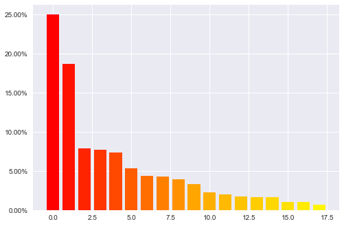
Show the distribution of a given data source
[4]:
distribution = metrics.get_distribution(items['genres'])
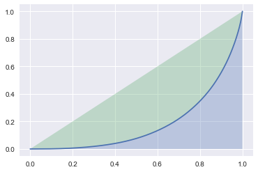
Draw a Lorenz curve graph for insights
Lorenz curve is a graphical representation of the distribution, the cumulative proportion of species is plotted against the cumulative proportion of individuals. This feature is also supported by rsdiv for helping practitioners’ analysis.
[5]:
metrics.get_lorenz_curve(ratings['movieId'])
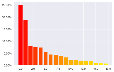
Show the distribution of a given data source
The unbalance of the data distribution can be well illustrated by both barplot and sorted DataFrame:
[6]:
distribution = metrics.get_distribution(items['genres'])
[7]:
distribution
[7]:
| category | count | percentage | |
|---|---|---|---|
| 0 | Drama | 1603 | 0.250156 |
| 1 | Comedy | 1200 | 0.187266 |
| 2 | Action | 503 | 0.078496 |
| 3 | Thriller | 492 | 0.076779 |
| 4 | Romance | 471 | 0.073502 |
| 5 | Horror | 343 | 0.053527 |
| 6 | Adventure | 283 | 0.044164 |
| 7 | Sci-Fi | 276 | 0.043071 |
| 8 | Children's | 251 | 0.039170 |
| 9 | Crime | 211 | 0.032928 |
| 10 | War | 143 | 0.022316 |
| 11 | Documentary | 127 | 0.019819 |
| 12 | Musical | 114 | 0.017790 |
| 13 | Mystery | 106 | 0.016542 |
| 14 | Animation | 105 | 0.016386 |
| 15 | Fantasy | 68 | 0.010612 |
| 16 | Western | 68 | 0.010612 |
| 17 | Film-Noir | 44 | 0.006866 |
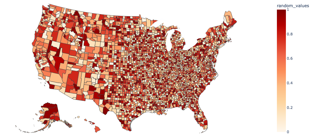
Evaluate the unbalance from a sense of location
rsdiv provides the encoders including geography encoding function to improve the intuitive understanding for practitioners, to start with the random values:
[8]:
import numpy as np

geo = rs.GeoEncoder()
df, gdict = geo.read_source()
rng = np.random.default_rng(42)
df['random_values'] = rng.random(len(df))
[9]:
geo.draw_geo_graph(df, 'random_values', 'name')
Data type cannot be displayed: application/vnd.plotly.v1+json